Variational Inference for Latent Variable Models
This post goes through the derivation of Evidence Lower Bound (ELBO) and an intuitive explanation of how variational inference works for latent variable models. Much of the intuition presented here is inspired by Sergey Levine’s lectures on variational inference and insights from discussions with Chris Heckman during my area exam.
Latent Variable Models
Suppose we want to model a complex data distribution \(p(x)\) given a dataset \(D = \{x_1, x_2, \ldots, x_N\}\) where \(x\) might represent images, robot trajectories, or other high-dimensional data. Directly modeling \(p(x)\) is often intractable due to its complexity.
Latent variable models address this challenge by introducing an auxiliary random variable \(z\) drawn from a simple distribution \(p(z)\), such as a Gaussian. Rather than modeling \(p(x)\) directly, we instead model how data is generated conditioned on the latent variable via \(p(x\vert z)\).
The conditional distribution \(p(x \vert z)\) is chosen to be easy to sample from. A common choice is also Gaussian:
\(\begin{equation} p(x \vert z) = \mathcal{N}(\mu(z), \sigma(z)) \end{equation}\),
where the mean \(\mu(z)\) and standard deviation \(\sigma(z)\) are functions of \(z\) learned from data. The marginal distribution over observations is then obtained by integrating out the latent variable:
\(\begin{equation} p(x) = \int p(x \vert z)p(z)dz \end{equation}\).
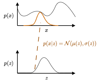
Sampling a latent variable \(z\) selects a Gaussian distribution over the data space via \(p(x \vert z)\). By drawing different values of \(z\) and sampling from the corresponding conditionals, the model can represent complex data distributions.
How do we train the model \(p_{\theta}(x)\)?
We can use maximum likelihood to train the model \(p_{\theta}(x)\) where \(\theta\) are the parameters of the model. However, the integration over \(z\) is intractable.
\(\begin{align} \mathcal{L}(\theta) &= \sum_{i=1}^{N} \log p_{\theta}(x_i) \\ &= \sum_{i=1}^N \log \int p(x_i\vert z)p(z)dz\\ \end{align}\).
Why is the integration over \(z\) intractable? The integration over \(z\) is intractable because \(p(x \vert z)\) depends nonlinearly on \(z\). In deep latent variable models, \(p(x \vert z)\) is typically parameterized as a Gaussian whose mean and variance are outputs of a neural netowrk.
\[\begin{equation} p(x \vert z) = \mathcal{N}(\mu_{nn}(z), \sigma_{nn}(z)) \end{equation}\]Because neural networks introduce nonlinear dependencies on \(z\), the integrand is no longer a Gaussian in \(z\), and the resulting integral has no closed-form solution.
Closed-form marginalization is only possible in restricted settings. For example, if \(p(z) = \mathcal{N}(0, I)\) and \(p(x \vert z) = \mathcal{N}(Az+b, \Sigma)\), then the model is linear-Gaussian, and the marginal distribution is \(p(x) = \mathcal{N}(b, AA^T + \Sigma)\).
What if \(z\) is discrete? If \(z\) were discrete, the integral would become a sum, but computing gradients of the log-likelihood would still require evaluating or summing over all latent states, which quickly becomes infeasible in large or structured latent spaces.
Why can’t we sample \(z\) to approximate the integral and gradients? We could approximate the marginal likelihood using Monte Carlo sampling: \(\begin{equation} p(x) \approx \frac{1}{M}\sum_{i=1}^M p(x \vert z_i), \quad z_i \sim p(z) \end{equation}\)
However, maximum likelihood requires gradients of \(\text{log}p(x)\) which depend on the posterior \(p(z \vert x)\). Sampling from the prior \(p(z)\) does not provide samples from the posterior. As a result, naive Monte Carlo sampling results in high variance estimates, leading to unstable and impractical learning. Below is the derivation for why \(\nabla_{\theta} \text{log}p_{\theta}(x)\) depends on \(p(z \vert x)\).
\[\nabla_{\theta} \text{log}p_{\theta}(x) = \frac{1}{p_{\theta}(x)} \nabla_{\theta} p_{\theta}(x) = \frac{1}{p_{\theta}(x)} \int \nabla_{\theta} p_{\theta}(x \vert z)p(z)dz\]Now, if we take the derivative of \(\text{log}p_{\theta}(x \vert z)\) with respect to \(\theta\), we get \(\nabla_{\theta} \text{log}p_{\theta}(x \vert z) = \frac{1}{p_{\theta}(x \vert z)} \nabla_{\theta} p_{\theta}(x \vert z)\). Then we get \(\nabla_{\theta}p_{\theta}(x \vert z) = p_{\theta}(x \vert z) \nabla_{\theta} \text{log}p_{\theta}(x \vert z)\). Substituting this into the gradient of \(\text{log}p_{\theta}(x)\), we get
\[\begin{equation} \nabla_{\theta} \text{log}p_{\theta}(x) = \frac{1}{p_{\theta}(x)} \int p_{\theta}(x \vert z) p(z) \nabla_{\theta} \text{log}p_{\theta}(x \vert z)dz \end{equation}\]We have the term \(\frac{p_{\theta}(x \vert z)p(z)}{p_{\theta}(x)}\), which is exactly the posterior \(p_{\theta}(z \vert x)\). The gradient becomes
\[\begin{align} \nabla_{\theta} \text{log}p_{\theta}(x) &= \int p_{\theta}(z \vert x) \nabla_{\theta} \text{log}p_{\theta}(x \vert z)p(z)dz\\ &= \mathbb{E}_{p_{\theta}(z \vert x)}\left[\nabla_{\theta} \text{log}p_{\theta}(x \vert z)\right] \end{align}\]Variational Approximation
This motivates the use of variational inference, which replaces the intractable posterior \(p(z \vert x)\) with a tractable approximation \(q_{\phi}(z \vert x)\) and yields a differentiable lower bound on the log-likelihood. Here we go through the derivation of the ELBO (Evidence Lower Bound). Starting with the log-likelihood which we want to maximize with respect to \(\theta\), we have
\[\begin{equation} \text{log}p_{\theta}(x) = \text{log} \int p_{\theta}(x \vert z)p(z)dz \end{equation}\]We introduce a variational distribution \(q_{\phi}(z \vert x)\), which is parameterized by \(\phi\) and approximates the posterior \(p_{\theta}(z \vert x)\). The key idea is to rewrite the marginal likelihood in a way that allows us to take expectations with respect to \(q_{\phi}(z \vert x)\), which we can sample from. We multiply the above equation by \(\frac{q_{\phi}(z \vert x)}{q_{\phi}(z \vert x)}\) and use the fact that \(\int q_{\phi}(z \vert x)dz = 1\) to get
\[\begin{align} \text{log}p_{\theta}(x) &= \text{log} \int p_{\theta}(x \vert z)p(z)dz\\ &= \text{log} \int p_{\theta}(x \vert z)q_{\phi}(z \vert x)\frac{p(z)}{q_{\phi}(z \vert x)}dz\\ &= \text{log} E_{z \sim q_{\phi}(z \vert x)}\left[\frac{p_{\theta}(x \vert z)p(z)}{q_{\phi}(z \vert x)}\right] \end{align}\]The logarithm is a concave function, so we can apply Jensen’s inequality to get
\[\begin{align} \text{log}p_{\theta}(x) &= \text{log} E_{z \sim q_{\phi}(z \vert x)}\left[\frac{p_{\theta}(x \vert z)p(z)}{q_{\phi}(z \vert x)}\right]\\ &\geq E_{z \sim q_{\phi}(z \vert x)}\left[\text{log}\frac{p_{\theta}(x \vert z)p(z)}{q_{\phi}(z \vert x)}\right]\\ &= \mathbb{E}_{z \sim q_{\phi}(z \vert x)}\left[\text{log}p_{\theta}(x \vert z) + \text{log}p(z) - \text{log}q_{\phi}(z \vert x)\right]\\ \end{align}\]The right hand side is the ELBO, which is a lower bound on the log-likelihood. It is a differentiable function of \(\theta\) and \(\phi\), and can be used to train the model.
What makes a good \(q_{\phi}(z \vert x)\)?
The intuition is that \(q_{\phi}(z \vert x)\) should be close to \(p(z)\), and we can use KL-divergence to measure the difference between the two distributions.
\[\begin{align} D_{KL}(q_{\phi}(z \vert x) \vert \vert p(z)) &= \mathbb{E}_{z \sim q_{\phi}(z \vert x)}\left[\text{log}\frac{q_{\phi}(z \vert x)}{p(z)}\right]\\ &= \mathbb{E}_{z \sim q_{\phi}(z \vert x)}\left[\text{log}q_{\phi}(z \vert x) - \text{log}p(z)\right] \end{align}\]So we can rewrite the ELBO as
\[\begin{align} \text{ELBO}(\theta, \phi) &= \mathbb{E}_{z \sim q_{\phi}(z \vert x)}\left[\text{log}p_{\theta}(x \vert z) + \text{log}p(z) - \text{log}q_{\phi}(z \vert x)\right]\\ &= \mathbb{E}_{z \sim q_{\phi}(z \vert x)}\left[\text{log}p_{\theta}(x \vert z) - D_{KL}(q_{\phi}(z \vert x) \vert \vert p(z)) \right] \end{align}\]To maximize \(p_{\theta}(x)\), we can maximize the ELBO with respect to \(\theta\) and \(\phi\). Intuitively, ELBO balances two objectives: the reconstruction loss \(\text{log}p_{\theta}(x \vert z)\) and the KL-divergence \(D_{KL}(q_{\phi}(z \vert x) \vert \vert p(z))\). The reconstruction loss encourages \(q_{\phi}(z \vert x)\) to place mass on latent variables that reconstruct \(x\) well, while the KL-divergence encourages \(q_{\phi}(z \vert x)\) to be close to \(p(z)\).
Enjoy Reading This Article?
Here are some more articles you might like to read next: