Minimizing Entropy for Classification Problems
When we want to be more confident about our predictions for a classification problem, we often use an objective that minimizes the entropy. But why is this not enough? This post will discuss entropy and cross entropy losses.
What is Entropy?
Entropy (in information theory) is a measure of uncertainty; the higher the entropy, the more uncertain you are. Entropy is defined as
\[H(X) = - \sum_{x \in \mathcal{X}} p(x)\text{log} p(x)\]where \(X\) is the discrete random variable that takes values in the alphabet \(\mathcal{X}\) and is distributed according to \(p: \mathcal{X} \rightarrow [0, 1]\). \(-\text{log}p(x)\) is the information of an event \(x\). So entropy \(H\) is the sum of the information for each possible event \(x \in \mathcal{X}\) weighted by the probability of the event \(p(x)\). Rare events (low probability) give more information and have higher values. Another way to think of it is that the entropy of a probability distribution is the optimal number of bits (when using log base 2) required to encode the distribution. When \(p(x)\) is high, we use fewer bits to represent the event \(x\) because we see it more often and it is cheaper to use fewer bits. When \(p(x)\) is low, we use more bits. This is given by the information of the event \(-\text{log}p(x)\).
Classification problems
In the context of human goal prediction, we want to train a model that outputs the correct human goal \(x\) given that the model observed some initial human trajectory \(\xi_{S \rightarrow Q}\) that started at point \(S\) and ended at point \(Q\). A human goal can be an object they are reaching towards or some task that they are performing. Suppose the human can reach towards the apple, banana, or grapes (\(\mathcal{X} = \{\text{apple}, \text{banana}, \text{grapes}\}\)), and we have a model \(f\) that outputs a distribution over the likelihood of goals (via neural network with softmax output or a Bayesian classifier). We can get the predicted goal by taking the argmax of the distribution \(\hat{x} = \text{argmax}_{x} f(\xi)\).
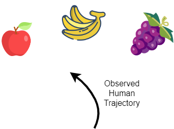
Grape icons created by Dreamcreateicons - Flaticon
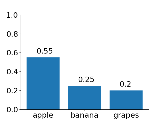
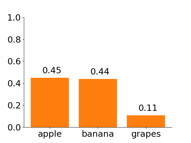
To train our model to be more certain about its predictions, we can minimize the entropy of the output distribution during training. We can use the following loss function: Given a predicted label \(\hat{x}\) and the true label \(x\), \(\mathcal{L}(x, \hat{x}) = \mathbb{1}\{x = \hat{x}\}H(f(x))+\mathbb{1}\{x != \hat{x}\}c\) for some constant \(c\). This equation penalizes the prediction by \(c\) if the prediction is incorrect and by the entropy if it is correct. \(\mathbb{1}\{q\}\) is the indicator function and evaluates to 1 if \(q\) is true otherwise 0. However, for predictions that are correct, minimizing the entropy may not give you more confident correct predictions. Suppose that the model has the following two predictions for the figure above where the human is reaching for the apple: 1) [0.55, 0.25, 0.2] and 2) [0.45, 0.44, 0.11]. The array corresponds to the goal distribution for apple, banana, and grapes respectively. Intuitively, we prefer the first array because the model is more confident (\(55 \%\)) about the prediction. However, the entropy for 1) is 0.998 and for 2) is 0.963. Minimizing the entropy will move the model outputs closer to 2) [0.45, 0.44, 0.11].
Connection to Cross Entropy
A common loss function for classification problems is the cross entropy loss. The cross entropy of distribution \(q\) relative to another distribution \(p\) is defined as
\[H(p, q) = - \sum_{x \in \mathcal{X}} p(x)\text{log}q(x)\]Intuitively, it measures the average number of bits needed to encode the actual distribution \(p\) when using the distribution \(q\). We can rewrite \(H(p, q)\) as
\[\begin{align} H(p, q) &= - \sum_{x \in \mathcal{X}} p(x)\text{log}q(x)\\ &= -\sum_{x \in \mathcal{X}} p(x) (\frac{\text{log}q(x)}{\text{log}p(x)} \text{log}p(x))\\ &= -\sum_{x \in \mathcal{X}} p(x) \frac{\text{log}q(x)}{\text{log}p(x)} - \sum_{x \in \mathcal{X}} p(x) \text{log}p(x)\\ &= D_{KL}(p||q) + H(p) \end{align}\]The first term is the Kullback-Leibler (KL) divergence which measures how different the distributions \(p\) and \(q\) are, and the second term is the entropy of \(p\). In addition to minimizing entropy, the cross entropy loss minimizes the distance between the predicted and actual distributions which resolves the issue above.
Enjoy Reading This Article?
Here are some more articles you might like to read next: