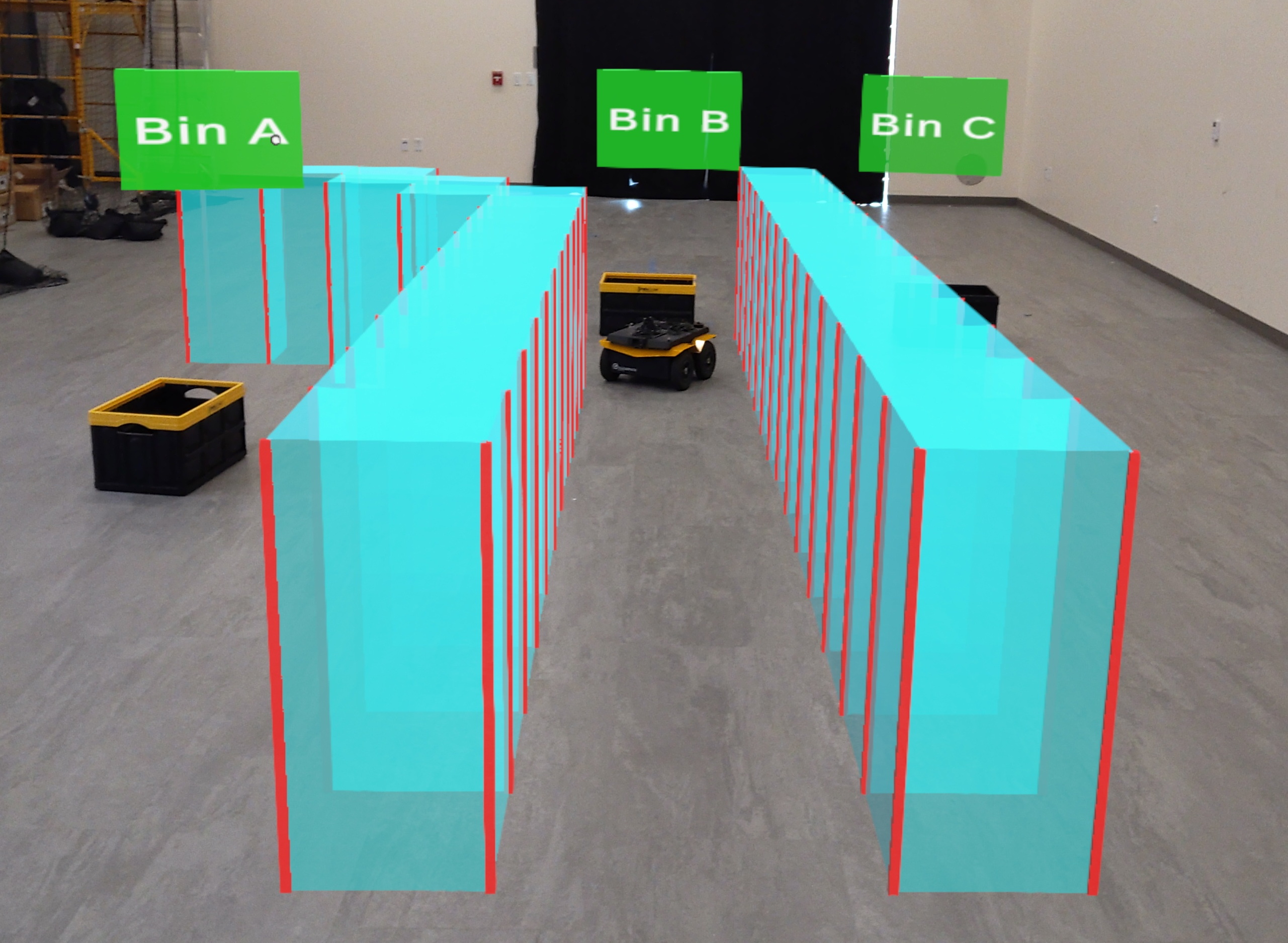
Figure 1.
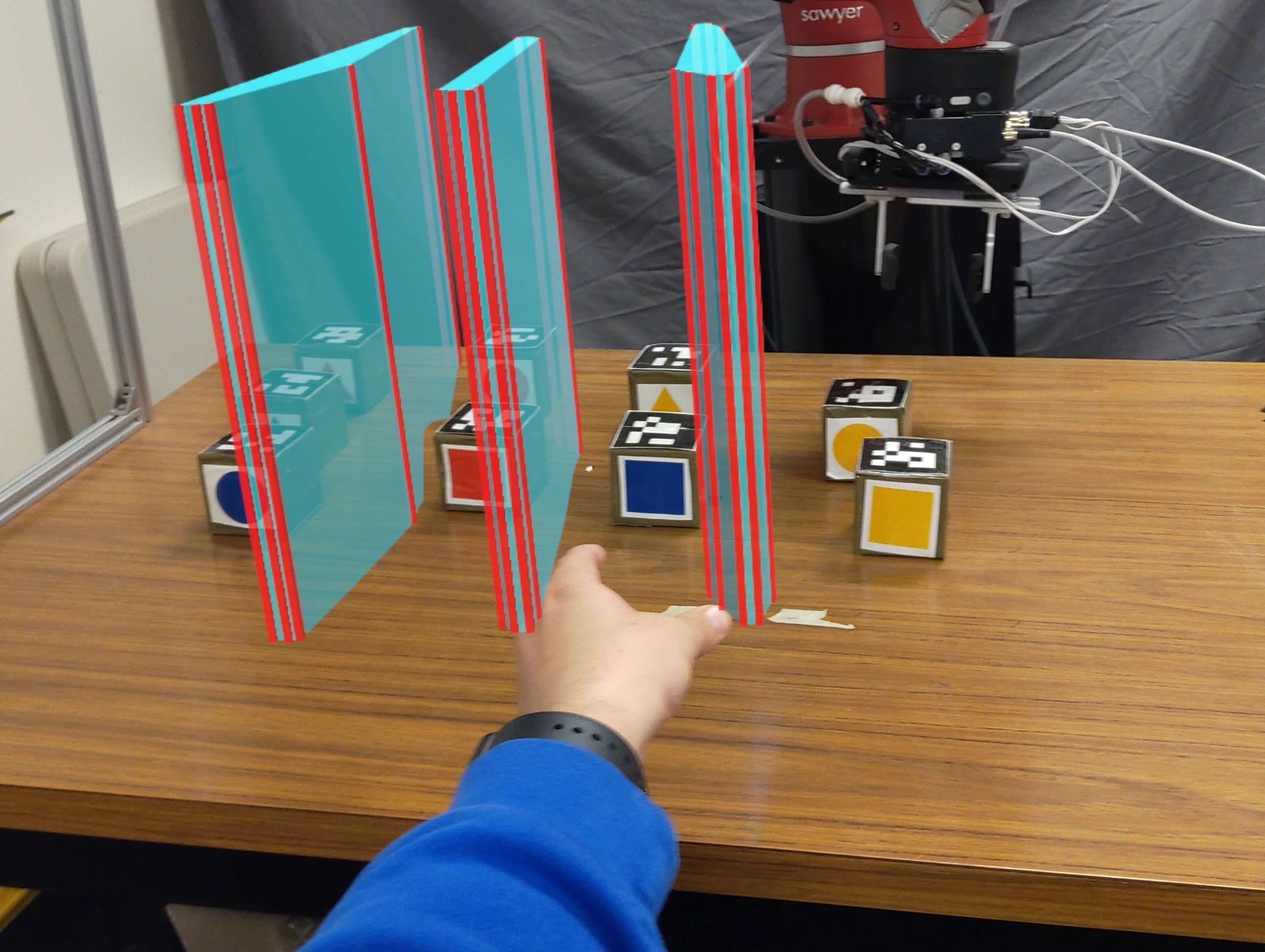
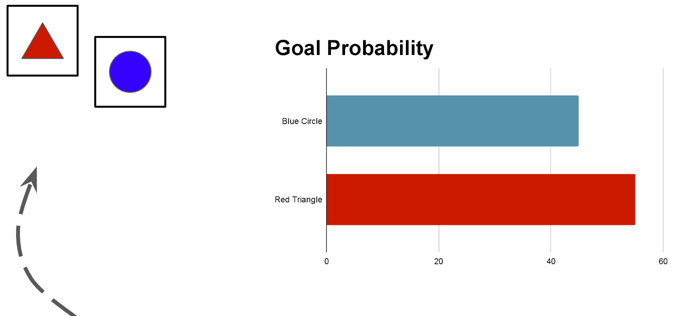
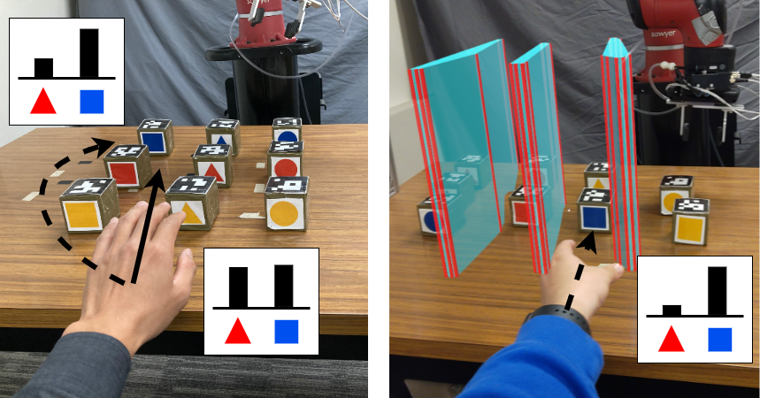
Suppose that you are picking up the blue square cube shown in Figure 1 (left). The natural path (solid) makes it hard for the robot to predict whether you are picking up the blue square cube or the red triangle cube while the legible path (dotted) requires you to take a circuitous route. To improve a robot's prediction of a human teammate's goals during a collaborative task shown in Figure 1 (right), the robot can configure the workspace by rearranging objects and projecting "virtual obstacles" in augmented reality (cyan and red barriers), in order to induce naturally legible paths from the human.
In human-robot collaboration, the robot needs to predict human motion in order to coordinate its actions with those of the human. Current algorithms rely on the human motion model to achieve safe interactions, but human motion is inherently highly variable as humans can always move unexpectedly. Our work takes a different approach and addresses a fundamental challenge faced by all human motion prediction models; we reduce the uncertainty inherent in modeling the intentions of human collaborators by pushing them towards legible behavior via environment design. Our work improves human motion model predictions by increasing environmental structure to reduce uncertainties, facilitating more fluent human-robot interactions.
Methods
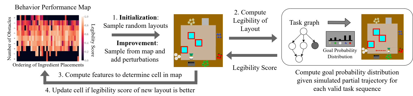
Figure 2.
Quality Diversity Search
We use a quality diversity (QD) algorithm called MAP-Elites to search through the space of environment configurations (i.e. object positions and virtual obstacle placements). MAP-Elites keeps track of a behavior performance map (also known as the solution map) that stores the best performing solution found for each combination of features chosen by the designer. For example, in the Overcooked game, we use two features 1) Number of Obstacles and 2) Ordering of Ingredient Placements. The environment shown in the middle of Figure 2 has 3 obstacles and ingredient ordering onions-fish-dish-tomatoes-cabbage. The solution map is a matrix where the first dimension is the number of obstacles and the second dimension includes the possible ingredient orderings. Note that the solution map can have more than 2 dimensions.
MAP-Elites consists of two phases: 1) initialization phase where environments are randomly generated and placed into the solution map according to their features and 2) improvement phase where environments are randomly sampled from the map and mutated. While MAP-Elites generates diverse solutions by altering existing ones through random mutations, the process may require substantial computational time to yield high quality solutions. Differentiable QD is a method that performs gradient descent on the objective function and the features to speed up MAP-Elites but requires both the objective and feature functions to be differentiable. We empirically approximate the gradient of the objective function through stochastic sampling, which may lead to “suboptimal” solutions that can, however, contribute to increased diversity. In our implementations, we continue this stochastic hill climbing until a local maxima is found. In Overcooked, we sample new locations for ingredients and additions/removals of virtual obstacles as possible mutations. The solution map is updated if the new environment generated from the mutation step is better than the existing solution in the solution map with the same features.
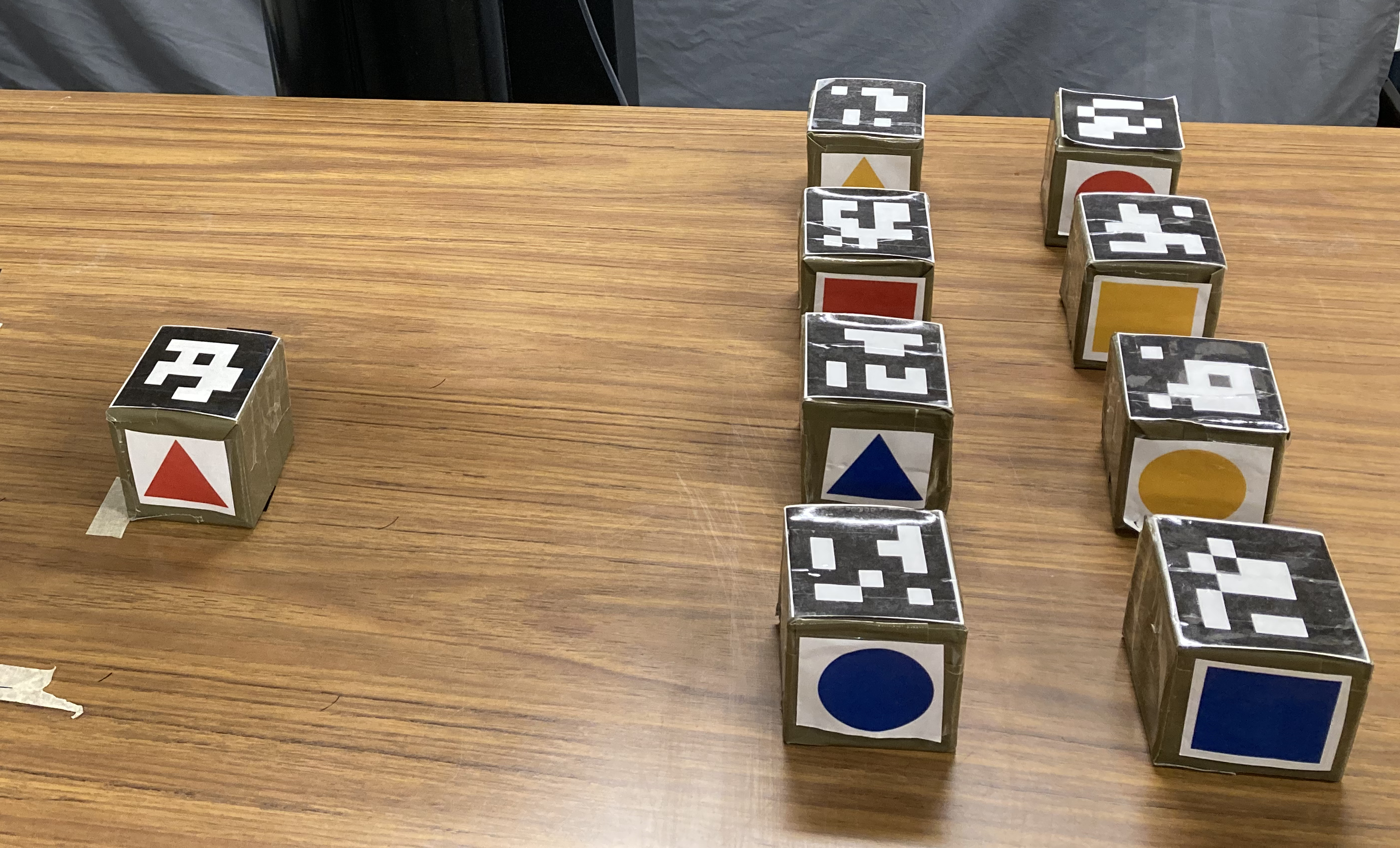
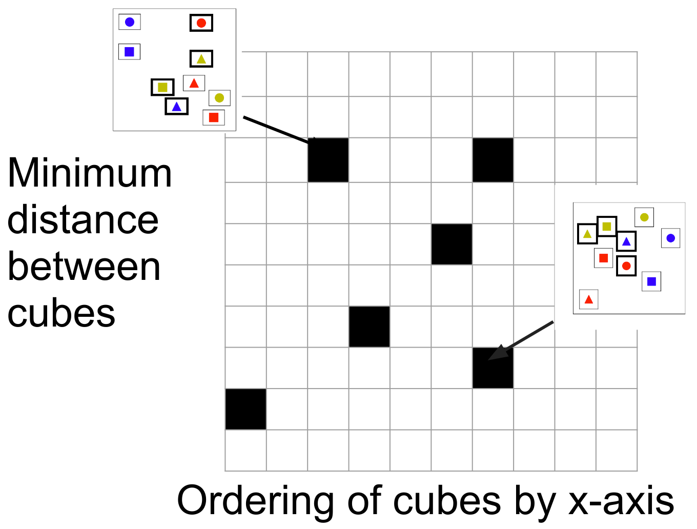
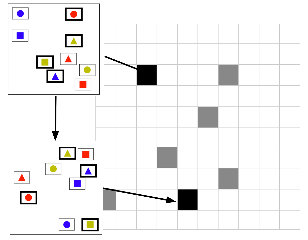
Figure 3.
The tabletop task in Figure 1 requires the human and the robot to collaboratively place cubes into a desired configuration shown in Figure 3 (left). To mutate an existing environment, we sample new locations for the cubes based on a Gaussian with variance = 7cm. We also sample the locations and orientations of fixed-size virtual obstacles. An example of the stochastic hill climbing in the improvement phase of MAP-Elites is shown in Figure 3 (right).
Legibility Objective Function
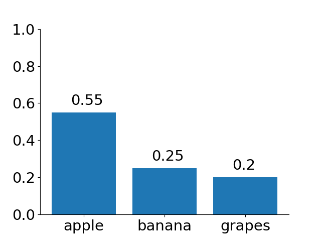
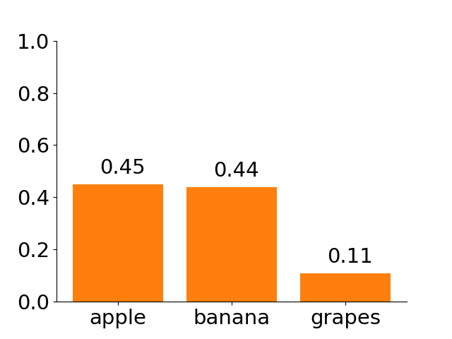
The objective function considers all the possible goals the human might be reaching for at a given stage of task execution and maximizes the probability of correctly predicting the human’s chosen goal. The probability of the human’s goal is given by the equation below:
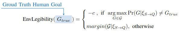
\[\Pr(G | \mathcal{\xi}_{S \rightarrow Q}) \propto \frac{exp(-C(\mathcal{\xi}_{S \rightarrow Q}) - C(\mathcal{\xi}^*_{Q \rightarrow G}))}{exp(-C(\mathcal{\xi}^*_{S \rightarrow G}))}\]The optimal human trajectory from point \(X\) to point \(Y\) with respect to cost function \(C\) is denoted by \(\mathcal{\xi}^*_{X \rightarrow Y}\). This equation evaluates how cost efficient (with respect to \(C\)) going to goal \(G\) is from start state \(S\) given the observed partial trajectory \(\mathcal{\xi}_{S \rightarrow Q}\) relative to the most efficient trajectory \(\mathcal{\xi}^*_{S \rightarrow G}\). For a given ground truth goal \(G_{true}\), if the predicted goal is not \(G_{true}\), we penalize by a constant \(c\) multiplied by the length of the observed trajectory \(\vert \mathcal{\xi}_{S \rightarrow Q} \vert\). If the predicted goal is correct, we encourage more confident predictions by maximizing the difference between the probability of the correct goal and the second highest goal probability. This is summarized in the equation below.
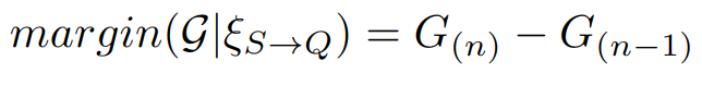
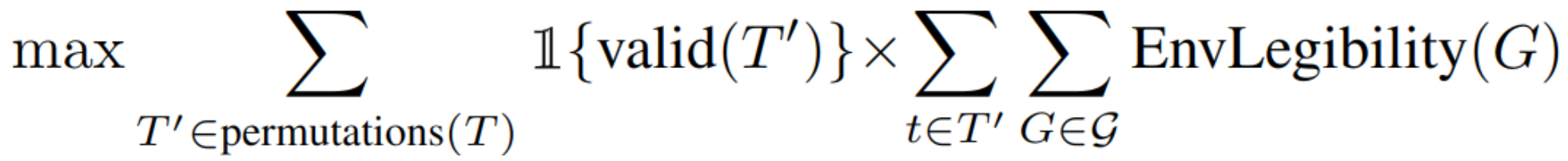
\[\text{EnvLegibility}(G_{true}) = \begin{cases} -c |\mathcal{\xi}_{S \rightarrow Q}|, \text{ if } \underset{G \in \mathcal{G}}{\arg\max} \Pr(G | \mathcal{\xi}_{S \rightarrow Q}) \neq G_{true} \\ margin(\mathcal{G}|\mathcal{\xi}_{S \rightarrow Q}) = G_{(n)} - G_{(n-1)}, \text{ otherwise} \end{cases}\]We compute EnvLegibility for each possible ground truth goal at each stage of the task execution. The function \(permutations(T)\) are all the different ways a task \(T\) can be performed. \(\mathcal{G}\) is the set of valid goals the human can reach for when performing subtask \(t\) with task ordering \(T'\).
\[\text{objective function} = \sum_{T' \in \text{permutations}(T)} \mathbb{1}\{\text{valid}(T')\} \times \sum_{t \in T'} \sum_{G \in \mathcal{G}} \text{EnvLegibility}(G)\]Experiments and Results
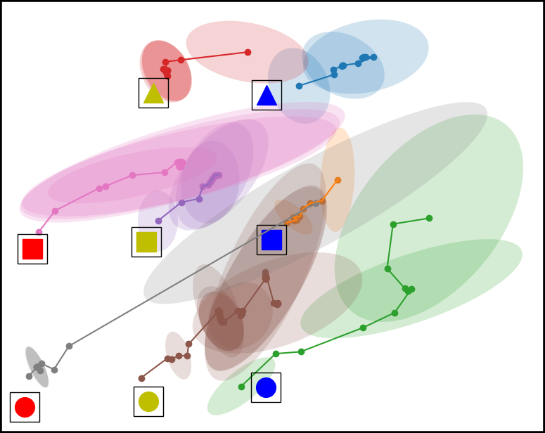
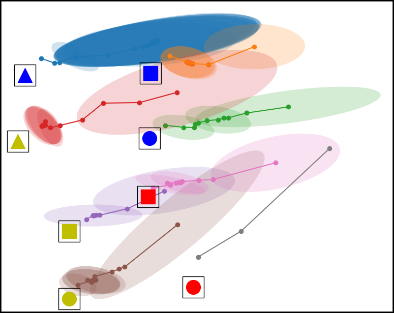
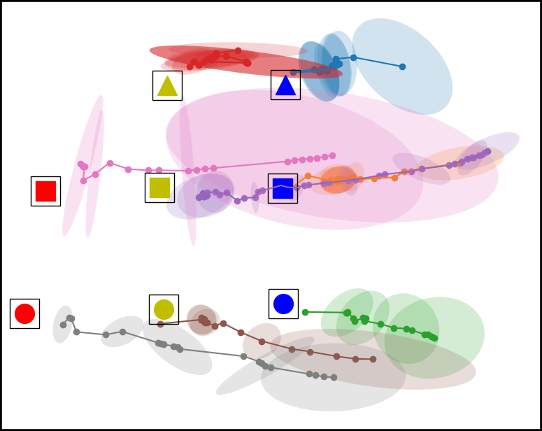
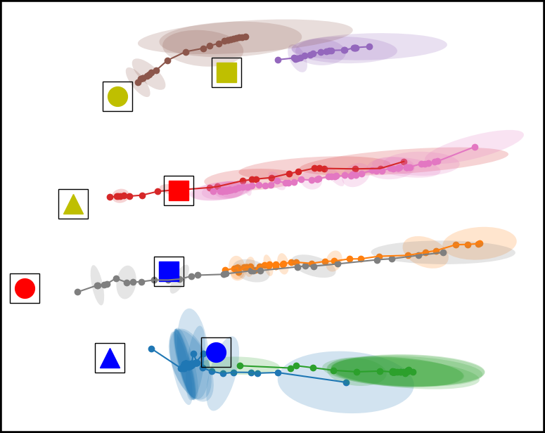
Figure 4. Top down view of the workspace plotting the mean and covariance of the time series multivariate Gaussian for each condition. From left to right, the conditions are Baseline, Placement Optimized, Virtual Obstacle Optimized, and our approach Both Optimized. The model in the Both Optimized condition has less covariance compared to the models trained in the other environment configurations.
Discussion
In this work, we introduce an algorithmic approach for autonomous workspace optimization to improve robot predictions of a human collaborator’s goals. We envision that our framework can improve human robot teaming, by improving goal prediction and situational awareness, for domains such as shared autonomy for assistive manipulation, warehouse stocking, cooking assistance, among others. Our approach is applicable for domains where the following conditions hold: 1) Multiple agents share the same physical space and the agents do not have access to other agents’ controllers or decision making processes (otherwise a centralized controller can be used), 2) the environment allows physical or virtual configurations, and 3) environment configuration can be performed prior to the interaction. Through dual experiments in 2D navigation (see paper) and tabletop manipulation, we show that our approach results in more accurate model predictions across two distinct goal inference methods, requiring less data to achieve these correct predictions. Importantly, we demonstrate that environmental adaptations can be discovered and leveraged to compensate for shortfalls of prediction models in otherwise unstructured settings.
]]>